NOTE: This is a working document that is regularly being edited and added to.
As noted in our discussion of both the quadrupole mass filter and quadrupole ion trap, in the late 1950's and early 1960's, Wolfgang Paul and collaborators were developing novel methodolgies for storing and manipulating ions through the use of alternating radio frequency electric fields. Their methodologies utilized quadrupolar fields, which by definition have potentials that scale with the square of x,y and z in a cartesian coordinate system:
$$\begin{equation}\phi(x,y,z) = A(\lambda x^2 + \sigma y^2 + \gamma z^2) + C\end{equation}$$
Because of the Laplace equation/condition, the gradient of the potential must equal zero (at least in the absence of any charges):
$$\begin{equation}\nabla\phi(x,y,z) = 2A(\lambda x + \sigma y + \gamma z) = 0\end{equation}$$
$$\begin{equation}\lambda x + \sigma y + \gamma z = 0\end{equation}$$
This equation can be satisfied in an infinite number of ways, with various values of the coefficients $\lambda$, $\sigma$ and $\gamma$. The linear ion trap (LIT) utilizes the combination $\lambda$=1, $\sigma$=-1 and $\gamma$=0 to give a potential of:
$$\begin{equation}\phi(x,y,z) = A(x^2 - y^2) + C\end{equation}$$
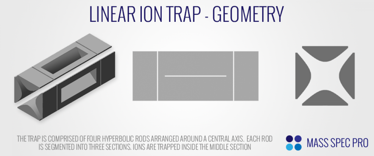
If this is looking familiar, it is because this is the exact same potential that is generated in the quadrupole mass filter (QMF). Just like the QMF, the ideal LIT field is generated by four hyperbolic rods arranged around a center axis:
The "x electrodes" have the form:
$$\begin{equation}x^2 - y^2 = r_0^2\end{equation}$$
and the "y electrodes" have the form:
$$\begin{equation}y^2 - x^2 = r_0^2\end{equation}$$
Note that in the most common variant of the LIT, the four rods are each segmented into three sections, as will be discussed later. In order to determine what the coefficients 'A' and 'C' are, we must consider the boundary conditions of the electrode surfaces themselves. For example, assume that there is a potential $\phi_0$ applied between the two rod sets, with $\frac{\phi_0}{2}$ applied to the x-electrodes and an opposite potential $\frac{-\phi_0}{2}$ applied to the y-electrodes. The equal and opposite voltages cancel out in the center of the rods, giving a value of C=0 in the potential:
$$\begin{equation}\phi(x,y) = A(x^2 - y^2)\end{equation}$$
The innermost point of the x-electrodes is located at $x=r_0$ and y=0, and has a potential of $\frac{\phi_0}{2}$:
$$\begin{equation}\phi(r_0,0) = \frac{\phi_0}{2} = Ax^2 = Ar_0^2\end{equation}$$
This gives a value of A:
$$\begin{equation}A = \frac{\phi_0}{2r_0^2}\end{equation}$$
A similar examination of the potential on the y-electrodes gives the same value for A. As such, the general potential in the LIT has the form:
$$\begin{equation}\phi(x,y) = \frac{\phi_0(x^2 - y^2)}{2r_0^2}\end{equation}$$
Now that we have determined the form of the potential as a funciton of x and y, we can consider what happens with the potentials that are usually applied to LITs. These potentials have both a static DC component and a time varying RF component:
$$\begin{equation}\phi_0 = 2(U + Vcos\Omega t)\end{equation}$$
Remember that $\phi_0$ is typically the difference in potential between the rods, which have equal and opposite potentials applied. This means that the DC component (2U) is split, such that one pair of rods has a DC component of +U and the other pair has -U. Likewise, the RF component $\left(2Vcos\Omega t\right)$ is split between the rods; this is accomplished by applying sinusoids of equal and opposite amplitude (V and -V) to the rod pairs. With all these considerations applied, one set of rods has the potential $+\left(U + Vcos\Omega t\right)$ applied while the other has the potential $-\left(U + Vcos\Omega t\right)$ applied.
Ion Motion in a Quadrupolar Field
Let's consider the motion of an ion in the x dimension, specifically with an ion on the x-axis (y=0). The potential along this axis is:
$$\begin{equation}\phi(x,0) = \frac{\phi_0 x^2}{2r_0^2}\end{equation}$$
The electric field along the x-axis at this point is the derivate of the potential:
$$\begin{equation}E_x = \frac{d\phi}{dx} = \frac{\phi_0 x}{r_0^2}\end{equation}$$
The force acting on the ion along this axis is determined by multiplying the electric field by -e:
$$\begin{equation}F_x = -eE_x = \frac{-e\phi_0 x}{r_0^2}\end{equation}$$
The classic equation F=ma can be applied here:
$$\begin{equation}F_x = ma = m\frac{d^2x}{dt^2} = \frac{-e\phi_0 x}{r_0^2}\end{equation}$$
Now we can insert the usual form of $\phi_0 = 2(U + Vcos\Omega t)$:
$$\begin{equation}m\frac{d^2x}{dt^2} = \frac{-2e(U + Vcos\Omega t) x}{r_0^2}\end{equation}$$
In preparation for what's to come, this equation is slightly rearranged:
$$\begin{equation}m\frac{d^2x}{dt^2} = -\left(\frac{2eU}{r_0^2} + \frac{2eVcos\Omega t}{r_0^2}\right) x\end{equation}$$
$$\begin{equation}\frac{d^2x}{dt^2} + \left(\frac{2eU}{mr_0^2} + \frac{2eVcos\Omega t}{mr_0^2}\right) x = 0\end{equation}$$
Interestingly, this equation of ion motion has the form of the "Mathieu equation", which is:
$$\begin{equation}\frac{d^2u}{d\xi^2} + \left(a_u -2q_ucos2 \xi \right)u=0\end{equation}$$
In order to make the equation of ion motion fit the Mathieu equation format exactly, we make the following substitutions:
$$\begin{equation}u=x\end{equation}$$
$$\begin{equation}\xi = \frac{\Omega t}{2}\end{equation}$$
$$\begin{equation}a_x = \frac{8eU}{mr_0^2 \Omega^2}\end{equation}$$
$$\begin{equation}q_x = \frac{-4eV}{mr_0^2 \Omega^2}\end{equation}$$
Similar considerations can be made for ion motion along the y-axis of the LIT, again providing an equation of motion that takes the form of a Mathieu equation with the values:
$$\begin{equation}a_y = \frac{-8eU}{mr_0^2 \Omega^2}\end{equation}$$
$$\begin{equation}q_y = \frac{4eV}{mr_0^2 \Omega^2}\end{equation}$$
Since the equation of ion motion along the x-axis of the LIT fits the form of the Mathieu equation, we can utilize known characteristics of said equation to think about ion trajectories inside the trap. The solutions to the Mathieu equation can be characterized as either "bounded" or "unbounded", based on how their amplitudes evolve over time. There are only certain combinations of $a_u$ and $q_u$ that provide bounded/stable solutions. As such, there are only certain values of $a_x$, $q_x$, $a_y$, and $q_y$ that provide stable ion trajectories.
When considering whether a solution is bounded (aka "stable") or unbounded (aka "unstable") in the x and y axes, it is useful to think in terms of a unitless variable $\beta_u$, which is a continued fraction of the values $a_u$ and $q_u$. For a given pair of q and a values, $\beta$ can be approximated as:
$$\begin{equation}\beta_u = \left[a_u - \frac{(a_u-1)q_u^2}{2(a_u-1)^2-q_u^2} - \frac{(5a_u+7)q_u^4}{32(a_u-1)^3(a_u-4)} - \frac{(9a_u^2+58a_u+29)q_u^6}{64(a_u-1)^5(a_u-4)(a_u-9)}\right]^\frac{1}{2}\end{equation}$$
Although this is a rather complicated relationship with q and a, the value of $\beta_u$ has a direct correlation to the stability (or lack thereof) of a solution. For values of $\beta_u$ between 0 and 1, solutions are stable in the respective dimension, and for all other values the solution is unstable. While this is not strictly true, it is sufficient for this discussion. For visualization of this concept, a "stability diagram" is often used:
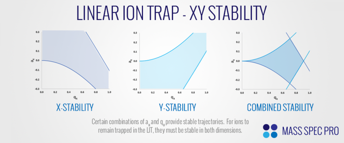
On the left side of the figure, the lines $\beta_x = 0$ and $\beta_x=1$ are represented as solid lines, with the space between them shaded in. This represents the combinations of a and q that provide stable solutions in the x dimension. For values of $q_x$ and $a_x$ outside of this region, the solution is unstable in the x-dimension. Likewise, the curves in the center graph represent $\beta_y = 0$ and $\beta_y = 1$, which bound the regions of stability in the y dimension. This particular graph can be confusing, because its axes are $q_x$ and $a_x$, despite being a plot of y-axis stability. As such, its shape is inverted vertically due to the sign difference between $a_x$ and $a_y$ for a given set of operating conditions. At this point, we have mapped the combinations of $a_x$ and $q_x$ that provide stable/bounded solutions in both the x and y dimensions. In order for ions to remain trapped by the LIT's fields, they must of course have stable trajectories in both dimensions. As such, it is only the region of overlap between x and y-stability that is of interest to us. This region is demonstrated in the rightmost graph. Generally speaking, ions who fall into this region for a given set of trapping conditions (RF amplitude, DC voltage, etc.) will remain in the trap.
While the RF field traps ions in the x and y dimensions, it is not effective at confining the ions in the z-dimension (viz. the trap's long center axis). Confinement along this axis is accomplished by placing a different DC potential on the end sections of the trap that is "higher" than the DC component of the center sections. For example, if the four rods of the center section all have a DC component of 0 Volts and positive ions are to be trapped, then the end sections must have a positive DC component. This potential difference creates an electric field that prevents ions from exiting along the trap's long axis.

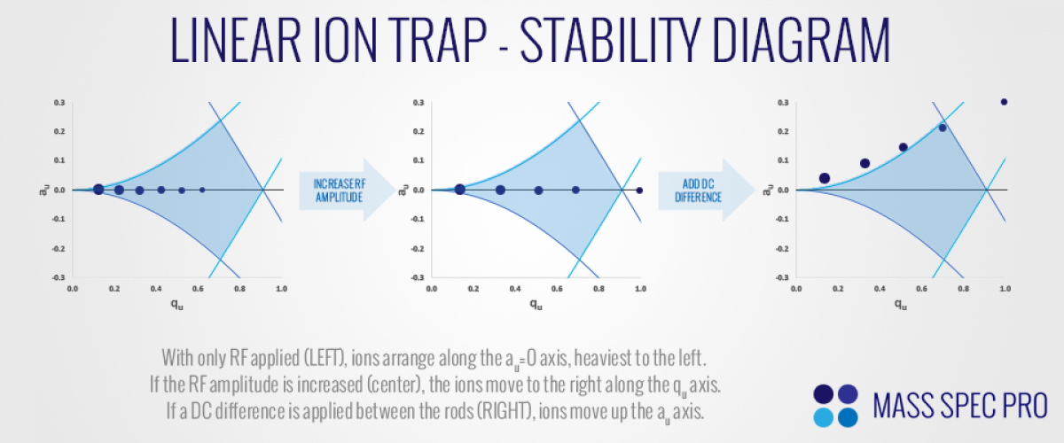
Now that we understand the basics of trap operation, we can consider the position of ions inside the stability diagram under different experimental conditions, namely different values of DC (U) and RF (V) voltages. First, consider the situation in which no DC is applied (U=0) and some RF apmlitude, V. According to equations 22 and 24, all ions will posses $a_u$ values of zero, regardless of their mass. Furthermore, according to equations 23 and 25, all ions will have non-zero $q_u$ values, with the heaviest ions having the lowest values and lightest ions having the highest values. As such, the ions arrange themselves along the $a_u=0$ line of the stability diagram, with the heaviest ions to the left (near $q_u=0$), and lighter ions offset to the right due to their different m values. If the RF amplitude is increased, the q-values of the ions will scale proportionally, moving them further to the right of the stability diagram. Then if a DC voltage is applied, the ions will move along the $a_u=0$ axis. According to equations 22 and 24, the degree to which they move is inversely proportional to their mass, with the heaviest ions remaining closer to the axis and lighter ions deviating further up the stability diagram:
In the right graph of the figure above, note how one of the masses is positioned just under the "apex" of the stability region, while all other masses are outside of the region. This is akin to how quadrupole mass filters (QMFs) work, with heavier ions being unstable in one dimension and lighter ions being unstable in the other dimension. While this mode of operation/isolation is certainly possible within the fields of an LIT, it is not common to manipulate ions in such a way. Rather ions are commonly shuttled around on the $a_u = 0$ axis by changing by changing the RF amplitude, V. In fact, ions can be mass analyzed and ejected from the LIT simply by changing the RF amplitude....
In the early 1908's, a team of scientists and engineers led by George Stafford at Finnigan developed a groundbreaking method of operating the QIT (the predecessor to the LIT). The method, described in US Patent #4540884, has since been coined "mass selective instability mode". This same methodology has since been adapted to the LIT. First, the trap is first filled with ions while RF is applied to the rods. A range of m/z values will have stable trajectories, based on the various experimental conditions (e.g. RF frequency, amplitude, ion m/z, etc.). Once a sufficient number of ions has been accumulated in the LIT's trapping volume, the ions are subsequently pushed to the right on the stability diagram by a linear ramp of the RF amplitude. This causes ions to cross over the stability boundary at $q_x = q_y = 0.908$ in order of increasing m/z. Since the ions are crossing over both the x and y stability boundaries, they become unstable in both directions simultaneously. As such, they can eject through small slits in both sets of rods:

Ion Motion
The motion of ions along each axis of a two-dimensional pure quadrupole field are completely independent/decoupled. Whatever happens to the ion's motion in the x-dimension has no effect on its motion in the y-direction and vice versa. Ion motion along each axis is rather complex, comprising numerous sinusoidal components in both dimensions. The frequencies of these components are termed "secular" frequencies, and they are related to the value of $\beta_u$ by:
$$\begin{equation}\omega_{u,n} = \left(n+\frac{1}{2}\beta_u\right)\Omega~~~~~~~~~~0\leq n < \infty \end{equation}$$
$$\begin{equation}\omega_{u,n} = -\left(n+\frac{1}{2}\beta_u\right)\Omega~~~~~~~~~~-\infty < n < 0\end{equation}$$
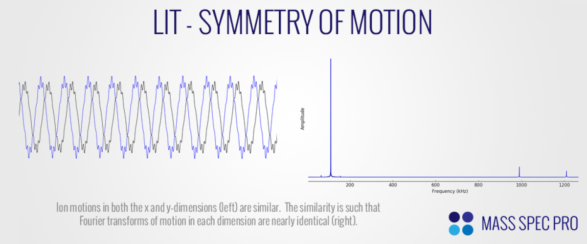
Since the integer 'n' can range from zero to $\pm \infty$ there are a large number of secular frequencies in any given ion's motion. However, generally speaking the relative strength of each secular frequency drops very quickly from $n=0$ to $n=\pm 1$, $n=\pm 2$, etc. Since the "fundamental" (n=0) frequency is the strongest component of a given ion's motion, the term "secular frequency" is typically used to describe this frequency alone. Since the dominant frequency of ion motion is at a lower frequency than the corresponding higher order components, an ion's motion comprises a low amplitude ripple on top of a more slowly varying sine wave:

It should be noted that ion motion in both the x and y-dimensions is similar in a 2D quadrupolar field like the LIT due to the symmetry of the fields. For example, the frequency components of ion motion are nearly identical for both axes, with essentially just a phase difference between them.
Since the secular frequency in both the x and y dimensions is a function of $\beta_x$ (and $\beta_y$), ions with different m/z values will possess different secular frequencies for a given RF amplitude. Likewise, as the RF amplitude changes, the secular frequencies of all ions in the trap change accordingly. It should also be noted that the maximum possible secular frequency that an ion will ever obtain is $\Omega/2$, occuring at the stability boundary:

PSEUDOPOTENTIAL MODEL
Since the main component of ion motion in the LIT (and its rotationally symmetric sibling, the QIT) is a sine wave, it was recognized in the late 1950's and early 1960's that ions could be approximated as oscillating in a harmonic "pseudopotential well". Even though the electric field of the LIT is oscillating rapidly with time, its time-averaged effect is essentially a pseudopotential with a restoring force pushing ions toward the center of the trap. The depth of this pseudopotential well is effectively a measure of how strongly an ion is confined within the trap. Well depth is the same in both the x and y dimensions, given by:
$$\begin{equation}\overline{D_{x,y}} = \frac{Vq_{x,y}}{4}\end{equation}$$
Several things should be noted about potential well depths:
- For a given RF amplitude, ions of high m/z will be sitting in shallower potential wells than their lighter counterparts due to their lower q values.
- For an ion of a given m/z, the potential well depth can be increased by raising the RF amplitude. The deeper well pushes the ions closer to the center line of the trap.
- If the RF amplitude is sufficiently low that an ion resides in a very shallow potential well, it could strike the electrodes and be neutralized. Under such conditions ions have a similar chance of being lost in either the x or y-dimension due to equal well depths.
- If a higher RF frequency is used, and the amplitude is scaled accordingly (to keep an ion at the same q value), ions will reside in deeper potential wells. In other words, higher RF frequencies can translate to stronger trapping of ions.
RESONANCE EJECTION/EXCITATION
Once an ion is confined within the trap by the RF voltage applied to the rods (in addition to the DC on the endcaps), the ion's motion can be excited by applying additional waveforms to the rods. The ion can pick up energy from the additional fields, causing it to move further away from the center of the trap. If considering the pseudopotential model, you can think of the ion as being pulled/pushed further up the sides of the potential well. If the ion's motion is excited sufficiently, the ion can either be ejected or strike an electrode. How is this excitation accomplished?
Perhaps the most common methodology is called "dipolar" excitation, in which a low amplitude AC field is applied between one of the rod pairs (with a frequency at or below Ω/2). Specifically, a low amplitude sine wave is applied to one rod, while an equal-and-opposite (180 degrees out of phase) sine wave is applied to the opposing rod. If the frequency of these waveforms closely matches the secular frequency of a given m/z, the ion will begin to "resonate" with the additional field, moving further and further from the center of the trap with a linear increase in amplitude with time.

The ability to excite an ion's motion and move it away from the center of the trap is one of the most powerful aspects of ion trap operation in mass spectrometry. It is used in several common modes of operation:
- Resonance Ejection: All commercial ion traps use some variant of "resonance ejection", in which they utilize AC waveforms to eject ions from the trap during the mass analysis step. Most commonly, bipolar excitation is performed during a linear ramp of the main trapping voltage. As ions move left to right across the stability diagram, their secular frequencies continually increase. Eventually their secular frequency approaches the biploar AC's frequency, and the ions begin to resonate and move further from the trap center. Eventually the ions have picked up enough energy to eject form the trap altogether. If done appropriately, resonance ejection can enhance the instrument's mass resolution (in comparison to normal "boundary ejection").
- Broadband Isolation: When performing MS/MS analysis with an ion trap, it is imperative to first isolate the m/z of interest. All other m/z values can be ejected from the trap by performing resonance excitation with a range of AC frequencies. If done appropriately (viz. with the correct frequencies omitted), a relatively narrow m/z range can remain in the trap while all others are ejected.
- Fragmentation: As ions move away from the center of the trap, they pick up kinetic energy. In the event that they subsequently collide with a neutral, there is an elevated amount of energy which can be converted into internal energy. If enough of these collisions occur, the ion can attain sufficient internal energy to actually break bonds, resulting in fragmentation. Such fragmentation can be achieved with resonance excitation by applying just enough amplitude to stretch the ion away from the center of the trap without actually ejecting it. This is critical for MS/MS, which requires both isolation and fragmentation.
ION CREATION/INJECTION
Ion traps have to be "filled" with ions prior to peforming mass analysis. This filling can be accomplished in one of two ways: creating ions directly within the trap or injecting ions into the trap. These are commonly referred to as "internal ionization" and "external ionization", respectively. Internal ionization is most often accomplished by leaking analyte neutrals into the ion trap volume and then firing a beam of electrons into the trapping volume while RF is applied. If the electrons are fired through the slits in the rods perpendicular to the trap's center axis, the fate of the electrons depends on the phase angle of the RF waveform. During the negative swing of the RF the electrons are repelled and possibly may not even enter the trap. However, during the positive swing of the RF many electrons will be accelerated into the trapping volume. If the electrons pick up sufficient kinetic energy, then their collisions with analyte neutrals will cause ionization. Since the newly made analyte ions are generated inside the trap, the RF field is able to confine the ions, focusing them to the center of the trap where they can be further manipulated/analyzed. It should be noted that internal ionization is only really applicable to volatile analytes. For lower volatility analytes, external ionization must be utilized.
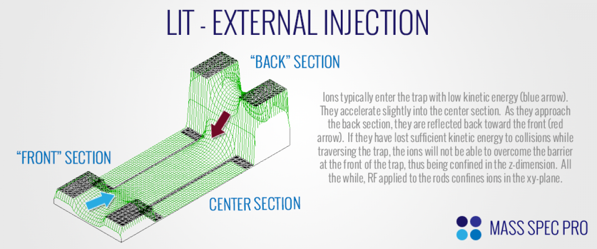
For external ionization instruments, a beam of ions is generated outside of the trap through another mechanism (e.g. electrospray, chemical ionization, etc.) and is then injected into the trap. Conventionally, the ion beam is injected along the centerline of the trap (z-axis). While RF is applied to the rods in order to confine ions in the xy-plane, we rely on DC fields between the trap segments to trap the ions in the z-dimension. During injection, the DC on the "front" segment of the trap is held just above the center segment of the trap, while the DC of the "back" segment of the trap is held considerably higher. As ions enter the trap, they are accelerated slightly by the potential drop between the front and center sections. Likewise, as ions approach the back segment of the trap they lose kinetic energy and reverse direction back towards the front of the trap. In an collision-free high vacuum chamber, the ions would pass right back out of the trap, overcoming the potential increase between the center and front sections. However, if they ions have lost some kinetic energy in the z-dimension due to collisions within the trap, they won't be able to overcome the potential barrier. As such, they will reflect toward the back of the trap and will now oscillate back and forth in the z-dimension, losing more kinetic energy with each successive collision they experience.
The LIT's trapping efficiency can be quite high, especially compared to its sibling, the QIT. When injecting into a QIT, the an ion passes through a hole in a grouned endcap and then begins to feel the potential applied to the "ring" electrode. The fate of the ion depends strongly on the phase angle of the ring's RF waveform. If the RF is on a positive swing when a positive ion enters the trap, said ion is repelled back into the endcap and neutralized. Conversely if the RF is on a negative swing when the ion enters, it will be accelerated rapidly through the trap, making it nearly impossible to trap. As a result, there are only narrow time windows within each RF cycle during which ions can be successfully trapped in a QIT. This phase angle dependence does not exist with the LIT, assuming it has bipolar RF applied. The equal and opposite RF waveforms on opposing rods cancel out along the centerline of the trap (where ions are injected). As such, the ions do not experience the push/pull of oscillating RF in the z-dimension, meaning they are equally likely to be trapped regardless of the RF phase when they enter the trap.
AUTOMATIC GAIN CONTROL (AGC)
For both internal and external ionization, the duration of "filling" can be adjusted as desired. If an insufficient number of ions is trapped, the fill time can be lengthened on the next scan to build up a larger population (e.g. to achieve higher SNR). Likewise, if too many ions are trapped, the fill time can be dynamically shortened on the next scan to mitigate the side effects (e.g. space charge repulsion between ions). This is yet another unique feature of ion traps. When an instrument is in the middle of a large spike in signal, it can throttle fill time down, providing improved dynamic range on the high end. Then as signal dies down, the instrument can throttle fill time back up, providing ultimate sensitivity and dynamic range on the low end. Essentially, AGC provides a mechanism that can balance both maximum sensitivity and dynamic range on the fly. This concept was pioneered by Finnigan Corporation in the late 1980's, and is often referred to as AGC (Automatic Gain Control). The original US patent (5107109) can be found here. Similar methodologies have been implemented by other vendors for their ion trap instruments as well.
HIGHER ORDER FIELDS
The previous discussion has assumed that the field inside the ion trap is 100% quadrupolar. However, it is physically impossible to generate such a field. There are several causes of non-quadrupolar field components within ion traps:
- Electrodes do not extend to infinity
- Slits in endcaps for ion ejection
- Imperfect machining of electrodes
- Imperfect alignment of electrodes
We can account for the non-quadrupolar components by realizing that the actual field can be modeled as a sum of various "multipole" fields. In other words, the field is a sum of quadrupole, hexapole, octopole, decapole, etc. components:
$$\begin{equation}\Phi(x,y) = \Phi_0\sum_{n=0}^{\infty}A_n\phi_n(x,y)\end{equation}$$
The value of "n" is the "order" of each multipole; n=2 is the quadrupole, n=3 is the hexapole, etc. The coefficient $A_n$ is a weighting factor for each multipole; the smaller the value, the less that multipole contributes to the overall field inside the trap. The value of $\phi_n(x,y)$ is the specific electric field distribution associated with each multipole, and is given by:
$$\begin{equation}\Phi_N(x,y) = \frac{Re[(x+iy)^n]}{r_0^n}\end{equation}$$
The equations for n=0 through n=6 have the form:
$$\begin{equation}\phi_0(x,y) = 1\end{equation}$$
$$\begin{equation}\phi_1(x,y) = \frac{x}{r_0}\end{equation}$$
$$\begin{equation}\phi_2(x,y) = \frac{x^2-y^2}{r_0^2}\end{equation}$$
$$\begin{equation}\phi_3(x,y) = \frac{x^3−3xy^2}{r_0^3}\end{equation}$$
$$\begin{equation}\phi_4(x,y) = \frac{x^4-6x^{2}y^{2}+y^4}{r_0^4}\end{equation}$$
$$\begin{equation}\phi_5(x,y) = \frac{x^5-10x^3y^2+5xy^4}{r_0^5}\end{equation}$$
$$\begin{equation}\phi_6(x,y) = \frac{x^6-15x^4y^2+15x^2y^4-y^6}{r_0^6}\end{equation}$$
$$\begin{equation}\phi_7(x,y) = \frac{x^7-21x^5y^2+35x^3y^4-7xy^6}{r_0^7}\end{equation}$$
$$\begin{equation}\phi_8(x,y) = \frac{x^8-28x^6y^2+70x^4y^4-28x^2y^6+y^8}{r_0^8}\end{equation}$$
The multipoles "above" quadrupolar are often referred to as "higher order fields". Any real-world ion trap has a predominantly quadrupolar field with small amounts of higher order multipoles overlayed on top of it. These higher order components can have very significant effects on ion motion:
- Motion along the axes are coupled: The separation of x and y motion from pure quadrupoles is not strictly true anymore. Kinetic energy can transfer back and forth between the two dimensions in complex ways.
- Motional frequencies depend on ion position: As ions move away from the centerline of the trap, their secular frequencies can increase or decrease depending on the nautre of the higher order fields. This can be advantageous in certain situations. For example, if secular frequency increases with ion amplitude, then it can actually assist resonance ejection. As the RF amplitude is ramped, the ion's secular frequency increases until it eventually approaches the resonance ejection frequency. As it begins to resonate, the ion's motional amplitude will increase. If the higher order fields then cause the secular frequency to increase, then the ion will move even closer to the resonance ejection frequency, causing it to eject even faster.
- Certain a,q combinations result in "non-linear resonances": Due to a complex interplay between the quadrupole and higher order fields, there are certain conditions that can cause ions to naturally pickup energy from the electric field. This can cause the ion's motional amplitue to increase significantly. The increased amplitude can be used as an advantage. For example, by performing resonance ejection at a non-linear resonance point, both the resonance ejection field and the naturally occurring non-linear resonance work in concert to eject ions faster than they would with resonance ejection alone.
Mass Resolution & Accuracy
The exact mass resolution and accuracy of an LIT depends on many inter-related variables, including scan rate, RF frequency, resonance ejection conditions, electrode quality, vacuum pressure, etc. However, it is generally safe to say that the LIT can provide "nominal mass" analysis capability. Peak widths are typically on the order of ~0.5 m/z, and mass accuracy is on the order of ~0.1-0.2 m/z, depending on the exact experimental conditions.
Comparison to Other Analyzers
Ion traps have several distinct advantages in relation to other mass analyzers. They are physically compact, have modest vacuum requirements, can scan relatively quickly and are capable of performing multiple stages of MS/MS all within a single volume. The LIT even has distinct advantages over its QIT sibling, namely its ability to trap ions more efficiently and to handle larger numbers of ions. The chief weakness of the LIT is its "nominal mass" resolution and accuracy, which limit its ability to distinguish between very subtle differences in mass.